Introduction and elimination for $~\forall$

With a richer language of symbols comes more rules that mimic how we argue about truth. Here we extend the rules of inference from propositonal logic to include rules for quantifiers and equality.

Introduction and elimination rules model how we use formulas as assumptions or conclude then as goals in arguments.

How would we conclude that something is true for all values of a variable? Let’s call our formula $A(x).$ Well, if we can establish $A(x)$ without imposing any “conditions” on $x$, we should be free to conclude $\forall x~ A(x)$. In particular, we should not have any hypotheses floating around that depend on $x$ themselves. For example, if we assumed that $4 \mid n$, then we could conclude that $n$ is even. But it would make no sense to conclude that $n$ is even for all $n$. Our standing assumption placed conditions on $n$.

Following this idea, we use the following introduction rule:

but only if $x$ is not free in any uncancelled hypotheses at this step.

Elimination works very much in the reverse. Given a proof of $\forall x~ A(x)$, we get a proof of $A(x)$ itself. A proof of a formula $A(x)$ with free variable behaves like a proof the formula of the universal quantification over it $\forall x~ A(x)$. We can be a more general

where $t$ is any other term available to us. You can think of this as a useful change of variables. However, we need to be careful about collisions of names – we need to make sure that $t$ is itself does not involve any variables bound elsewhere in $A(x)$. For example, if we have the formula $\forall x~ \exists~y \neg(x = y)$ and we try to eliminate to $\exists y~ \neg(y = y)$ by taking $t=y$ we quickly run into problems.

Introduction and elimination for $~\exists$

Now let’s think about the existential quantifier. If we can provide a proof of $A(t)$, now regardless of the extra assumptions, we can conclude $\exists x~ A(x)$.

Again our switch from $t$ to $x$ allows for convenient change of variables.

We next come to the existential elimination. It is a good point to stop and make a useful analogy between the pair $\forall$ and $\exists$ and the pair $\land$ and $\lor$. Suppose we our variable could only take a finite set of values $x_1,\ldots,x_n$. Then saying $\forall x~ A(x)$ is true is equivalent to saying that the big conjunction \(A(x_1) \land A(x_2) \land \cdots \land A(x_n)\) is true.

Similarly, saying that $\exists x~ A(x)$ is true is equivalent to the big disjunction \(A(x_1) \lor A(x_2) \lor \cdots \lor A(x_n)\) being true.

Via this analogy, in the general setting, $\forall$ can be viewed as akin to an “infinite and” and $\exists$ can be viewed as an “infinite or”. From within this interpretation, the elimination rule for $\exists looks familiar.

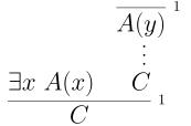
To use $\exists x~ A(x)$ in a proof and reach a conclusion $C$, we need to provide a proof that, in any case, we can prove $C$. Formally, we have

Like with $\lor$, we need to provide an argument in any case, $A(y)$, concluding $C$ to use the fact we know there is some $x$ such that $A(x)$ holds.

Rules for \(~=\)

Finally, we have a set of rules for $=$. While these do not look like our previous rules, they should seem familiar from experience. Equality allows us to build new formula, namely $x = y$.

First, we should know that $x=x$ always.

Next, we have that $=$ is symmetric.

And that $=$ is transitive.

Finally, we have two rules regarding subsitution into functions and predicates.

Equal inputs produce equal outputs of functions.

If we have equal terms and a proof a predicate depending on the first term, then we can conclude we have a proof of the same predicate after substitution.